Chapter 2 Data analysis and transformation

In this section, we analyze the various input features of the HIGGS dataset and apply deskewing and \(z\)-score normalization.

2.1 Momentum features

The input features containing _pT are related to transverse (perpendicular to the input beams) momentum, as is missing_E_mag. Histograms of these features are plotted as follows:

x |>
  select(c(contains('_pT'), 'missing_E_mag')) |>
  as.data.frame() |>
  gather() |>
  ggplot(aes(value)) +
  geom_histogram() +
  facet_wrap(~key, scales = "free", nrow = 2) +
  ggtitle('Momentum features')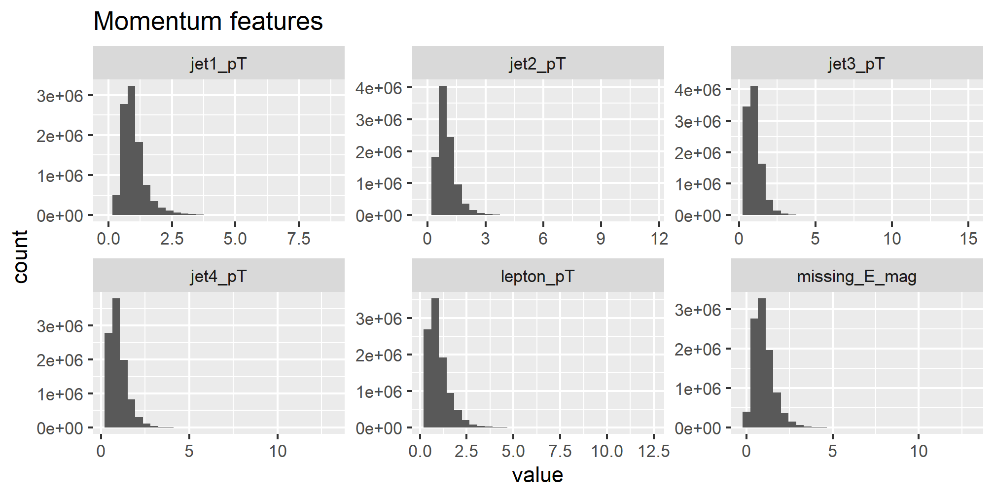

The momentum features are all quite skewed. To deskew the data, we apply a log transformation:

x |>
  select(c(contains('_pT'), 'missing_E_mag')) |>
  as.data.frame() |>
  log() |>
  gather() |>
  ggplot(aes(value)) +
  geom_histogram() +
  facet_wrap(~key, scales = "free", nrow = 2) +
  ggtitle('Momentum features (log transform)')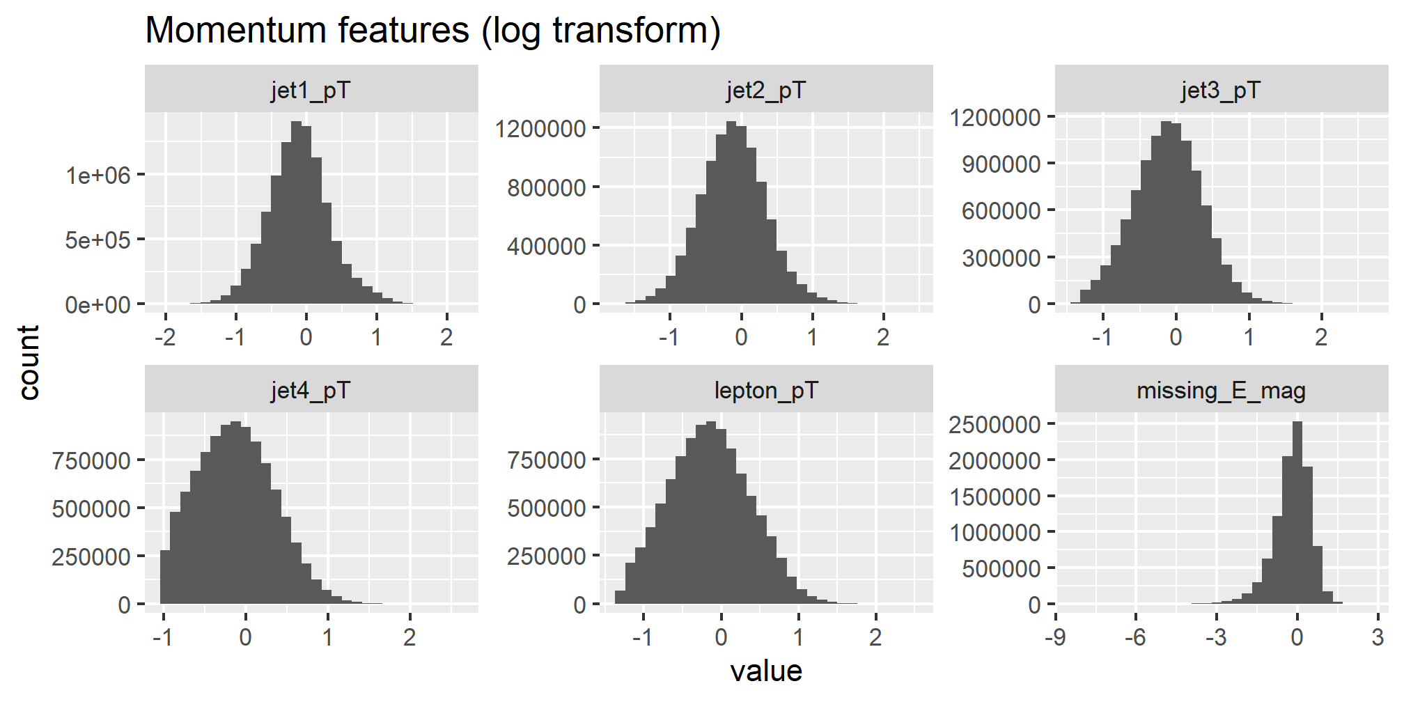

The skewness of the data before and after log transformation is as follows:

tibble(
  Feature = x |>
    select(c(contains('_pT'), 'missing_E_mag')) |>
    as.data.table() |>
    colnames(),
  Skewness = x |>
    select(c(contains('_pT'), 'missing_E_mag')) |>
    as.data.table() |>
    as.matrix() |>
    colskewness(),
  'Skewness (log)' = x |>
    select(c(contains('_pT'), 'missing_E_mag')) |>
    as.data.table() |>
    log() |>
    as.matrix() |>
    colskewness()
) |>
  kable(align = 'lrr', booktabs = T, linesep = '')

Feature	Skewness	Skewness (log)
lepton_pT	1.759399	0.1494493
jet1_pT	1.902766	0.1615350
jet2_pT	1.966270	0.0772273
jet3_pT	1.706359	0.0125490
jet4_pT	1.726289	0.2643133
missing_E_mag	1.487827	-0.8840618

2.2 Angular features

The features containing _eta or _phi describe angular data of the detected products of the simulated collision processes, in radians. Histograms for these features are as follows:

x |>
  select(c(contains('_eta'), contains('_phi'))) |>
  as.data.frame() |>
  gather() |>
  ggplot(aes(value)) +
  geom_histogram() +
  facet_wrap(~key, scales = "free_y", nrow = 3) +
  xlim(-pi,pi) +
  ggtitle('Angular features')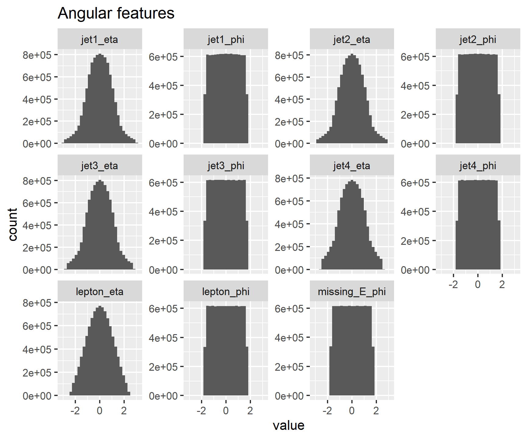

The histograms above do not show significant skew; therefore, deskewing will not be applied to these input features.

2.3 \(b\)-tag features

Each \(b\)-tag feature contains three possible values:

x |>
  select(contains('_btag')) |>
  as.data.frame() |>
  gather() |>
  ggplot(aes(value)) +
  geom_histogram() +
  facet_wrap(~key, scales = "free", nrow = 2) +
  ggtitle('b-tag features')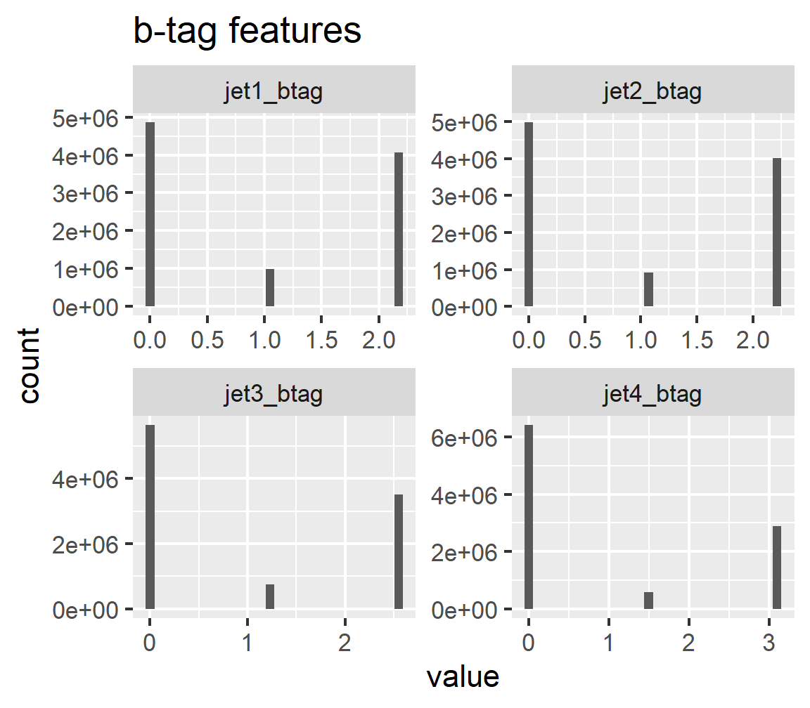

Interestingly, the \(b\)-tag data is encoded to have unit mean, but not unit standard deviation:

# b-tag means
tibble(
Mean = x |>
    select(contains('_btag')) |> 
    as.data.table() |> 
    as.matrix() |> 
    colMeans(),
'Standard Deviation' = x |>
    select(contains('_btag')) |> 
    as.data.table() |> 
    as.matrix() |> 
    colVars(std=T)
) |>
  rownames_to_column('Feature') |>
  kable(align = 'lrr', booktabs = T, linesep = '')

Feature	Mean	Standard Deviation
1	1.0000549	1.027791
2	1.0000157	1.049421
3	1.0000600	1.193689
4	0.9998079	1.400151

Nevertheless, we will leave these features alone.

2.4 High-level features

The high-level features for the HIGGS dataset are related to tranverse momentum and, as with the low-level momentum features, are quite skewed:

x |>
  select(contains('m_')) |>
  as.data.frame() |>
  gather() |>
  ggplot(aes(value)) +
  geom_histogram() +
  facet_wrap(~key, scales = "free", nrow = 3) +
  ggtitle('High-level features')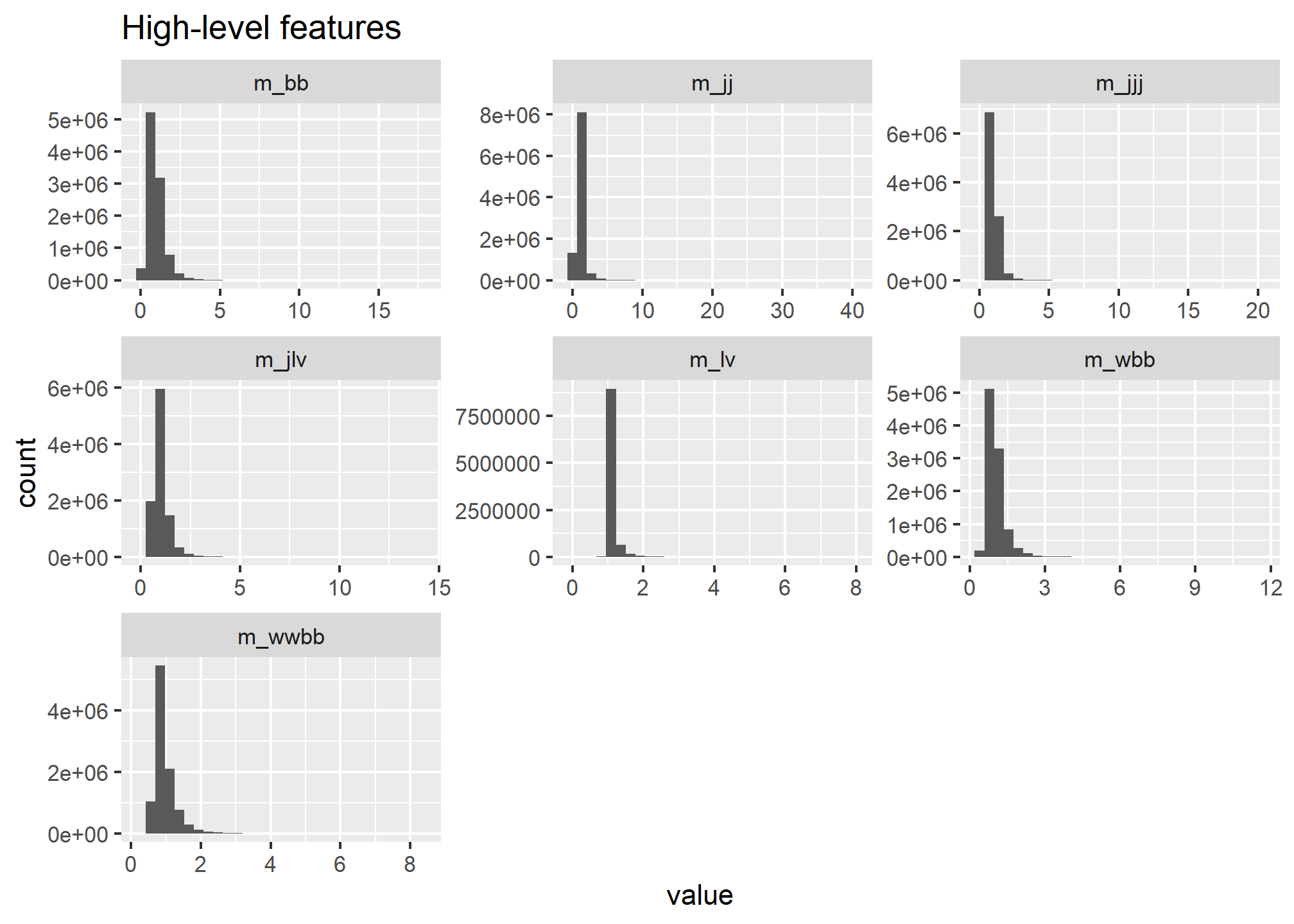

Therefore, we will apply a log transformation to this data:

x |>
  select(contains('m_')) |>
  as.data.frame() |>
  log() |>
  gather() |>
  ggplot(aes(value)) +
  geom_histogram() +
  facet_wrap(~key, scales = "free", nrow = 3) +
  ggtitle('High-level features (log transform)')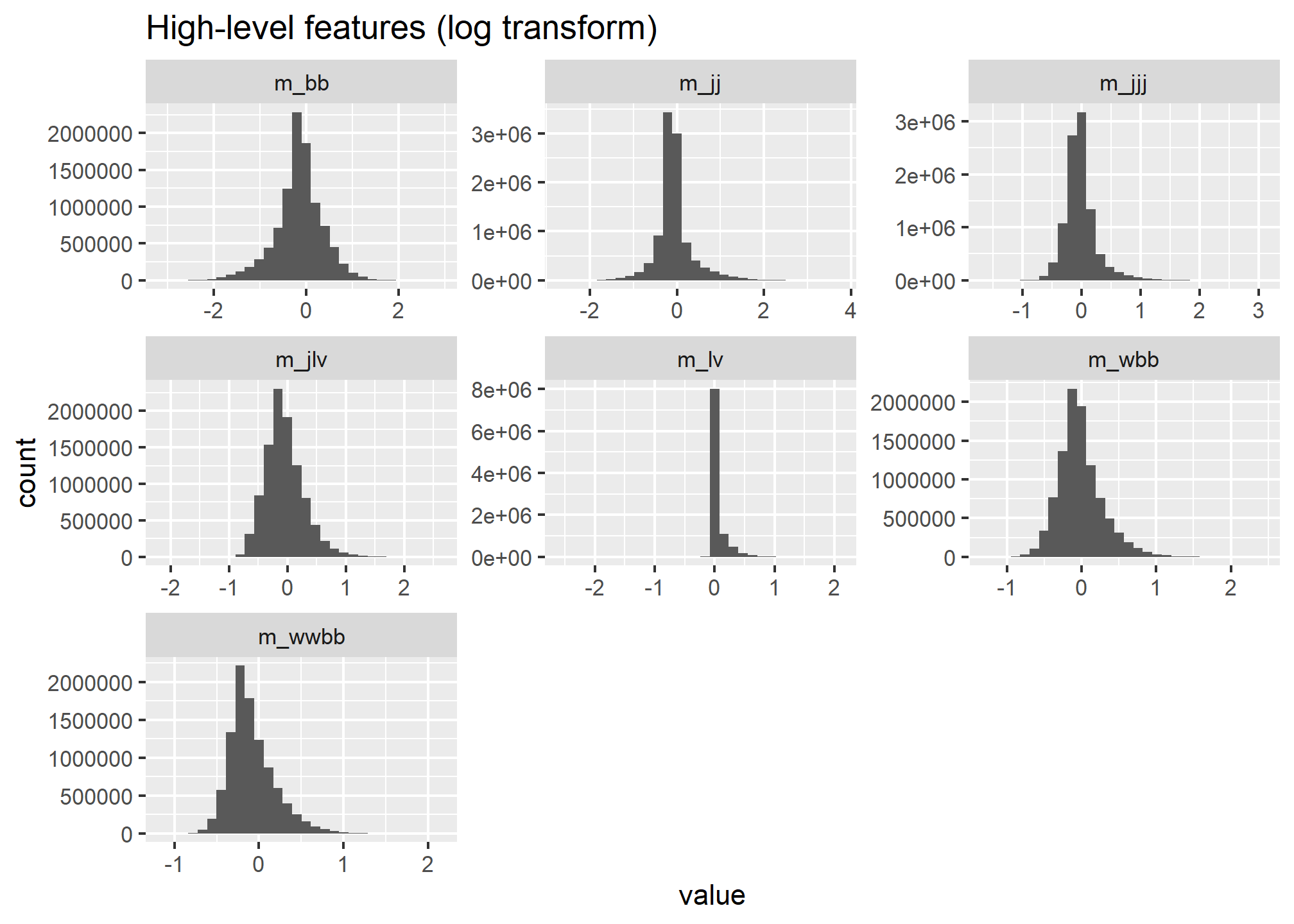

The skewness of the high-level features, before and after log transformation, are as follows:

tibble(
  Feature = x |>
    select(contains('m_')) |>
    as.data.table() |>
    colnames(),
  Skewness = x |>
    select(contains('m_')) |>
    as.data.table() |>
    as.matrix() |>
    colskewness(),
  'Skewness (log)' = x |>
    select(contains('m_')) |>
    as.data.table() |>
    log() |>
    as.matrix() |>
    colskewness()
) |>
  kable(align = 'lrr', booktabs = T, linesep = '')

Feature	Skewness	Skewness (log)
m_jj	6.529976	1.1279300
m_jjj	5.007659	1.4937149
m_lv	4.614399	2.9117405
m_jlv	2.850652	0.7598249
m_bb	2.424460	-0.3608753
m_wbb	2.687129	0.8387949
m_wwbb	2.548881	1.0247968

2.5 Final data transformation

The following code applies log transformation to selected columns of the HIGGS training and test datasets. We will also convert our data types into matrices here for input into subsequent stages of our analysis:

# Apply log transforms
x <- x |>
  mutate(
    across(
      c(contains('m_'), contains('_pT'), contains('_mag')),
      log
    )
  ) |>
  as.data.table()

xFinalTest <- xFinalTest |>
  mutate(
    across(
      c(contains('m_'), contains('_pT'), contains('_mag')),
      log
    )
  ) |>
  as.data.table()

# Convert to matrices
x <- x %>% as.matrix()
xFinalTest <- xFinalTest %>% as.matrix()

gc()

The following code then scales the training and final validation data to have zero mean and unit standard deviation:

m <- colMeans(x)
sd <- colVars(x, std = T) # std=T -> compute st. dev. instead of variance

x <- scale(x, center = m, scale = sd)
xFinalTest <- scale(xFinalTest, center = m, scale = sd)

Finally, we extract the target values to a vector:

y <- y$signal
yFinalTest <- yFinalTest$signal